Machine Learning Ex2 - Linear Regression

Andrew Ng has posted introductory machine learning lessons on the OpenClassRoom site. I’ve watched the first set and will here solve Exercise 2.

The exercise is to build a linear regression implementation, I’ll use R.

The point of linear regression is to come up with a mathematical function(model) that represents the data as best as possible, that is done by fitting a straight line to the observed data. This model will then allow us to make predictions on new data.

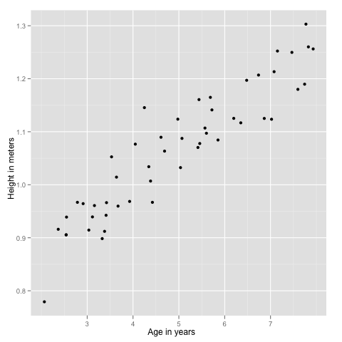
For example, the data we use here are boys ages and their corresponding heights, so when we get the mathematical model we will be able to guess the boys height from his age.

Data

google.spreadsheet <- function (key) {
  library(RCurl)
  # ssl validation off
  ssl.verifypeer <- FALSE

  tt <- getForm("https://spreadsheets.google.com/spreadsheet/pub", 
                hl ="en_GB",
                key = key, 
                single = "true", gid ="0", 
                output = "csv", 
                .opts = list(followlocation = TRUE, verbose = TRUE)) 

  read.csv(textConnection(tt), header = TRUE)
}

# load the data
mydata = google.spreadsheet("0AnypY27pPCJydDB4N3MxM0tENlk3UElnZ013cW1iM3c")

# include ggplot2
library(ggplot2)

ex2plot = ggplot(mydata, aes(x, y)) + geom_point() + 
       ylab('Height in meters') +
       xlab('Age in years')

Theory

The model we will get at the end is a line that fits the data, is defined like so:

Setting \(x_0 = 1\):

h_\theta(x) = \theta_0 x_0 + \theta_1 x_1 + \theta_2 x_2 + …

That can be summarized by (last is matrix notation):

h_\theta(x) = \sum_{i=0}^n \theta_i x_i = \theta^T x

Matrix representation is useful because has good support in software tools.

Goal is to get the line closest to observed data points as possible, thus we can define a cost function that returns the difference of the real data vs myModel:

J(\theta) = \frac{1}{2m} \sum_{i=1}^m (h_\theta(x^{(i)}) - y^{(i)})^2

where i is each data example we have and m is their total.

With J we now have a metric to check if the hypotheses line is getting closer to data points or not.

Next step is to find the smaller cost as possible from J, and in fact thats exactly what the gradient descent algorithm does: starting with an initial guess it iterates to smaller and smaller values of a given function by following the direction of the derivative:

x_i := x_{i-1} - \epsilon f^’ (x_{i-1})

Applying to our J:

\theta_j := \theta_j - \alpha \frac{\delta}{\delta \theta_j} J(\theta)

And doing a bit of calculus on derivatives we get:

\theta_j := \theta_j - \alpha \frac{1}{m} \sum_{i=1}^m (h_\theta(x^{(i)}) - y^{(i)}) x^{(i)}

Where alpha defines the size of steps of the convergence to \(\theta\).

Now lets check if all this math really works.

Implementation - take 1

alpha = 0.07
m = length(mydata$x)
theta = c(0,0)
x = mydata$x
y = mydata$y 
delta = function(x,y,th,m) {
  sum = 0
  for (i in 1:m) {
    sum = sum + (((t(th) %*% c(1,x[i])) - y[i]) * c(1,x[i]))
  }
  return (sum)
}

# 1 iteration
theta - alpha * 1/m * delta(x,y,theta,m)
       
          1
[1] 0.07452802 0.38002167

Implementation - take 2

After having a peek at the Matlab solution, i learned that is possible to replace the sum in the equation with a transpose matrix multiplication(like done with the line equation):

\theta := \theta - \alpha \frac{1}{m} x^T (x\theta^T - y)

So we can get a full matrix implementation:

alpha = 0.07
m = length(mydata$x)
theta = matrix(c(0,0), nrow=1)
x = matrix(c(rep(1,m), mydata$x), ncol=2)
y = matrix(mydata$y, ncol=1)
delta = function(x,y,th) {
  delta = (t(x) %*% ((x %*% t(th)) - y))
  return(t(delta))
}

# 1 iteration
theta - alpha * 1/m * delta(x,y,theta)



           [,1]      [,2]
[1,] 0.07452802 0.3800217

The Model

First we run several iterations, until convergence:

for (i in 1:1500) {
  theta = theta - alpha * 1/m * delta(x,y,theta)
}
theta

          [,1]       [,2]
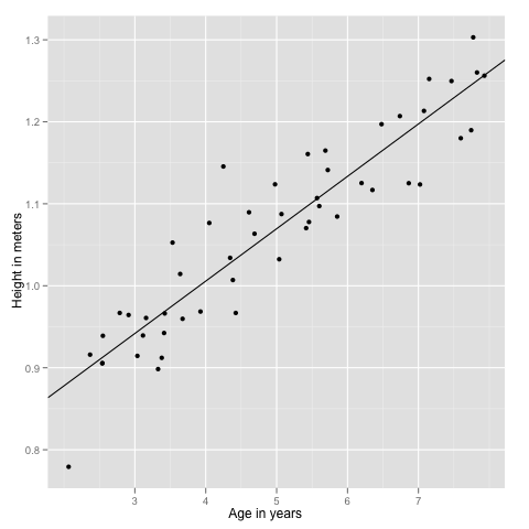
[1,] 0.7501504 0.06388338

And finally we see how well the line(model) fits the data:

ex2plot + geom_abline(intercept=theta[1], slope=theta[2])

References

• MATLAB / R Reference, by David Hiebeler
• Short Math Guide for LaTex(.pdf)
• Matrix multiplier tool

• Thanks to Andrew Ng and OpenClassRoom for the great lessons.