Weight Loss Predictor

Got for 2010 Xmas a very cool book called the “4 Hour Body”(thanks Jose Santos) written by Tim Ferriss who write a previous favorite of mine about productivity, the 4 hour work week.

I like the book’s approach, it doesn’t just say do this do that and you’ll be healthy, it actually says: I(Tim Ferriss) have tried this, exactly with these steps, during this time, this is how i measured, these are the results i got and by looking at most up-to-date medical research this is the most likely explanation for these results… Notice the similar principles of AB testing, as in, try things out and measure results, and see if they work for you.

Also, this book couldn’t have arrived in a better time as i just peeked my heaviest weight in a long time, blame it on [insert favorite reason]… so, long story short and I am now on the 3rd week of the low-carb diet described in the book.

But of course, like with all diets, I’m quickly growing impatient of when i’m going to reach my goal of adequate BMI, so lets use R and monte carlo simulations to generate predictions.

Data

Have been tracking my weight using google spreadsheets, so i can get the data into R like so:

google.spreadsheet <- function (key) {
  library(RCurl)
  # ssl validation off
  ssl.verifypeer <- FALSE

  tt <- getForm("https://spreadsheets.google.com/spreadsheet/pub", 
                hl ="en_GB",
                key = key, 
                single = "true", gid ="0", 
                output = "csv", 
                .opts = list(followlocation = TRUE, verbose = TRUE)) 

  read.csv(textConnection(tt), header = TRUE)
}

# load the data
mydata = google.spreadsheet("0AnypY27pPCJydEstZnVOeHYycjVWWktjbHpvS1NRMUE")

# Create a new column with the proper date format
mydata$timestamp = as.Date(mydata$timestamp, format='%d/%m/%Y')

The last 5 measurements:

tail(mydata, 5)

     timestamp   kg
140 2011-03-04 77.3
141 2011-03-05 76.9
142 2011-03-06 77.2
143 2011-03-07 77.3
144 2011-03-08 76.9

Past Years weight

Lets have a look at the weight fluctuations over the past 3,5 years(before diet).

# include ggplot2
library(ggplot2)

beforediet = subset(mydata, timestamp < "2011-01-18")
ggplot(beforediet, aes(x=timestamp, y=kg)) + geom_point() + geom_smooth() 

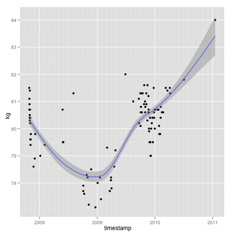
Weight has been mostly(in average) 80.5kg, but in 2nd half of 2010 we see a big jump. Also note that middle of year(summer here) appears to be where jumps in weight happen.

Predicting the Future

Now using Monte Carlo methods lets simulate the future based on the weight changes that happened since start of diet.

First we need to do some trickery to fill in the missing days and calculate the changes for every single day. The idea for filling in missing days is to interpolate between the known days and fill in the missing values. Eg: day1=81 and day3=80, we set day2=80.5.

So lets get the weight(kg) change(delta), for every day:

library(zoo) # for missing values interpolation

fill.all.days = function (mydata, timecolname, valuecolname) {
  dtrange = range(mydata[,timecolname])

  # create a data frame with every single day
  alldays = data.frame(tmp=seq(as.Date(dtrange[1]), as.Date(dtrange[2]), "days"))
  colnames(alldays) = c(timecolname) # rename tmp to proper timecolname

  # add the existing values
  alldays = merge(alldays, mydata, by=timecolname, all=TRUE)

  # fill in the missing ones
  alldays[,valuecolname] = na.approx(alldays[,valuecolname])
  return(alldays)
}

# from start of diet
dietdata = subset(mydata, timestamp >= "2011-01-17")
lastweight = tail(dietdata$kg, n=1)

# fill in missing days
dietalldays = fill.all.days(dietdata, "timestamp", "kg")

# get difference day by day into data frame
kgdelta = diff(dietalldays$kg)
dietalldays$delta = c(0, kgdelta)

# print only the 10 last values
tail(dietalldays, 5)    

    timestamp   kg delta
47 2011-03-04 77.3   0.0
48 2011-03-05 76.9  -0.4
49 2011-03-06 77.2   0.3
50 2011-03-07 77.3   0.1
51 2011-03-08 76.9  -0.4

What is going to be my weight in a week?

predict.weight.in.days = function(days, inicialweight, deltavector) {
  weight = inicialweight
  for (i in 1:days) {
    weight = weight + sample(deltavector, 1, replace=TRUE)
  }
  return(weight)
}

# simulate it 10k times
mcWeightWeek = replicate(10000, predict.weight.in.days(7, lastweight, kgdelta))

summary(mcWeightWeek)   

   Min. 1st Qu.  Median    Mean 3rd Qu.    Max. 
   71.8    75.2    75.9    75.9    76.6    79.7

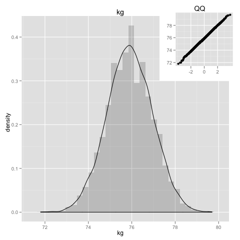
Another good thing about monte carlo methods is that they give a distribution of the prediction, so is possible to get a feeling of how sure the average is, by comparing it with a expected normal distribution:

gghist = function(mydata, mycolname) {
  pl = ggplot(data = mydata)
  subvp = viewport(width=0.35, height=0.35, x=0.84, y=0.84)

  his = pl + 
        geom_histogram(aes_string(x=mycolname,y="..density.."),alpha=0.2) + 
        geom_density(aes_string(x=mycolname)) + 
        opts(title = names(mydata[mycolname]))

  qqp = pl + 
        geom_point(aes_string(sample=mycolname), stat="qq") + labs(x=NULL, y=NULL) + 
        opts(title = "QQ")

  print(his)
  print(qqp, vp = subvp)
}

gghist(data.frame(kg=mcWeightWeek), "kg")

And when am i getting to 75kg?

days.to.weight = function(weight, inicialweight, deltavector) {
  target = inicialweight
  days = 0
  while (target > weight) {
    target = target + sample(deltavector, 1, replace=TRUE)
     days = days + 1
     if (days >= 1095) # if value too crazy just interrupt the loop
        break
  }
  return(days)
}

# simulate it 10k times
mcDays75 = replicate(10000, days.to.weight(75, lastweight, kgdelta))

summary(mcDays75)


   Min. 1st Qu.  Median    Mean 3rd Qu.    Max. 
   2.00    8.00   12.00   15.36   19.25  102.00

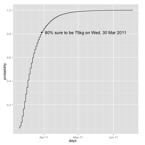
And the cumulative distribution:

# add dates to it, from today's date + #days
days75 = sort(tail(mydata$timestamp, 1) + mcDays75)

# get the ecdf values into a dataframe
days75.ecdf = summarize(data.frame(days=days75), days = unique(days), 
                        ecdf = ecdf(days)(unique(days)))

# date where its 80% sure i'll reach goal
prob80 = head(days75.ecdf[days75.ecdf$ecdf>0.80,],1)

# plot
ggplot(days75.ecdf, aes(days, ecdf)) + geom_step() +
       ylab("probability") + 
       geom_point(aes(x = prob80$days, y = prob80$ecdf)) +
       geom_text(aes(x = prob80$days, y = prob80$ecdf, 
                    label = paste("80% sure to be 75kg on",
                            format(prob80$days, "%a, %d %b %Y"))), 
                     hjust=-0.04)

Also note that, weight loss is faster at the beginning of a diet, it tends to slow down over time, so to keep the predictions valid we need to continue record the weight and re-run the predictions frequently.

But as you see the slow carb diet seems to work, even without exercise. Tim’s book is great, focusing on the smallest things possible for the bigger results(=efficiency).

Update

Got to 75.0kg on 25 March. Thats 67 days (aprox. 9 weeks) for a 9kg loss, thus aprox. 1kg per week. Which is within the recommended(0.9kg per week) weight loss recommendations. Thus am now within normal BMI values.

References

• Hard drive occupation prediction with R: part 1 and part 2, and thanks to Leandro Penz on the feedback.

• Big thanks for Jose and Tim, on jumpstarting this experiment!