
Machine Learning Ex3 - Multivariate Linear Regression
Exercise 3 is about multivariate linear regression. Start by finding a good learning rate (alpha) and then implement linear regression using the normal equations instead of the gradient descent algorithm.
With implementation in R.
Data
As usual hosted in google docs:
google.spreadsheet <- function (key) {
  library(RCurl)
  # ssl validation off
  ssl.verifypeer <- FALSE

  tt <- getForm("https://spreadsheets.google.com/spreadsheet/pub",
                hl ="en_GB",
                key = key,
                single = "true", gid ="0",
                output = "csv",
                .opts = list(followlocation = TRUE, verbose = TRUE))

  read.csv(textConnection(tt), header = TRUE)
}

# load the data
mydata = google.spreadsheet("0AnypY27pPCJydExfUzdtVXZuUWphM19vdVBidnFFSWc")
Feature Scaling
When applying the gradient descent, we need to make sure that features values are in the same order of magnitudes, otherwise it will not converge well, so here’s a helper function to scale features:
# given a data frame and the column names i want to scale
# creates new columns: feature.scale = (feature - mean)/std
feature.scale = function (dta, cols) {
  for (col in cols) {
    sigma = sd(dta[col])
    mu = mean(dta[col])
    dta[paste(names(dta[col]), ".scale", sep = "")] = (dta[col] - mu)/sigma
  }
  return(dta)
}

dta = feature.scale(mydata, c("area", "bedrooms"))
tail(dta, 5)


   area bedrooms  price area.scale bedrooms.scale
43 2567        4 314000  0.7126179      1.0904165
44 1200        3 299000 -1.0075229     -0.2236752
45  852        2 179900 -1.4454227     -1.5377669
46 1852        4 299900 -0.1870900      1.0904165
47 1203        3 239500 -1.0037479     -0.2236752
Finding Alpha
Recall from ex2 that the gradient descent equation for the updates of theta is:
\theta := \theta - \alpha \frac{1}{m} x^T (x\theta^T - y)
For finding a good alpha(\(\alpha\)) we will use a trial and error approach. The idea is look at how the Cost value \(J(\alpha)\) drops with the number of iterations, the fastest the drop the better, but if goes up then the alpha value is already too large.
The Cost is given by(in vectorized form):
J(\theta) = \frac{1}{2m} (X\theta - y)^T (X\theta - y)
See the lessons on details how to reach that equation.
Implementing:
# lets try out a few alpha's
alpha = c(0.03, 0.1, 0.3, 1, 1.3, 2)

# store the J values over the iterations
J = array(0,c(50,length(alpha)))
m = length(dta$price)
theta = matrix(c(0,0,0), nrow=1)
x = matrix(c(rep(1,m), dta$area.scale, dta$bedrooms.scale), ncol=3)
y = matrix(dta$price, ncol=1)

# the delta updates
delta = function(x,y,th) {
  delta = (t(x) %*% ((x %*% t(th)) - y))
  return(t(delta))
}

# the cost for a given theta
cost = function(x,y,th,m) {
  prt = ((x %*% t(th)) - y)
  return(1/m * (t(prt) %*% prt))
}

# run J for 50x, on each alpha
for (j in 1:length(alpha)) {
  for (i in 1:50) {
    J[i,j] = cost(x,y,theta,m) # capture the Cost
    theta = theta - alpha[j] * 1/m * delta(x,y,theta)
  }
}

# lets have a look
par(mfrow=c(3,2))
for (j in 1:length(alpha)) {
  plot(J[,j], type="l", xlab=paste("alpha", alpha[j]), ylab=expression(J(theta)))
}
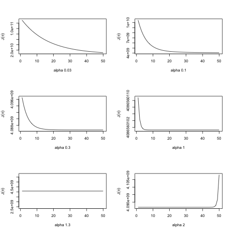
alpha 1 seems to be the best.
Setting \(\alpha=1\) and running until convergence:
# running until convergence
for (i in 1:50000) {
  theta = theta - 1 * 1/m * delta(x,y,theta)
  if (abs(delta(x,y,theta)[2]) < 0.0000001) {
    break # to interrupt updates
  }
}

# 1. The final values of theta
print("Theta:")
print(theta)

# 2. The predicted price of a house with 1650 square feet and 3 bedrooms.
# Don't forget to scale your features when you make this prediction!
print("Prediction for a house with 1650 square feet and 3 bedrooms:")
print(theta %*% c(1, (1650 - mean(dta["area"]))/sd(dta["area"]), (3 - mean(dta["bedrooms"]))/sd(dta["bedrooms"])))


 Warning message:
closing unused connection 3 (tt)
[1] "Theta:"
         [,1]     [,2]      [,3]
[1,] 340412.7 110631.1 -6649.474
[1] "Prediction for a house with 1650 square feet and 3 bedrooms:"
         [,1]
[1,] 293081.5
Normal Equations
Given the cost function:
J(\theta) = \frac{1}{2m} \sum_{i=1}^m (h_\theta(x^{(i)}) - y^{(i)})^2
Recall that this function returns how big is the error of our model vs the data. Thus our goal is to minimize it. And in order to find its minimum there is also a more direct approach (instead of using gradient descent) we can just calculate its derivative set it to 0 and find the value of theta:
\frac{\delta}{\delta \theta_j} J(\theta_j) = 0
thats for \(\theta_j\). We need of course to account for every j.
If we write it down into matrix notation, calculate its derivatives and set it to 0, then the value of theta will be obtained with:
\theta = (X^T X)^{-1} (X^T y)
That can be easily implemented like so:
x = matrix(c(rep(1,m), mydata$area, mydata$bedrooms), ncol=3)
y = matrix(mydata$price, ncol=1)
theta.normal = solve(t(x) %*% x) %*% (t(x) %*% y)

# 1. In your program, use the formula above to calculate. Remember that
# while you don't need to scale your features, you still need to add
# an intercept term.
print("Theta:")
print(theta.normal)

# 2. Once you have found  from this method, use it to make a price prediction
# for a 1650-square-foot house with 3 bedrooms. Did you get the same price
# that you found through gradient descent?
print("Price prediction for a 1650-square-foot house with 3 bedrooms")
t(theta.normal) %*%  c(1, 1650, 3)


[1] "Theta:"
           [,1]
[1,] 89597.9095
[2,]   139.2107
[3,] -8738.0191
[1] "Price prediction for a 1650-square-foot house with 3 bedrooms"
         [,1]
[1,] 293081.5
Normal equations are more direct but also more costly than gradient descent to run, so depending on situation you might need to choose one or the other.
References
- OpenClassroom Machine Learning
- Exercise 3: Multivariate Linear Regression
-
Thanks to Andrew Ng and OpenClassRoom for the great lessons.