Machine Learning Ex5.2 - Regularized Logistic Regression

Exercise 5.2 Improves the Logistic Regression implementation done in Exercise 4 by adding a regularization parameter that reduces the problem of over-fitting. We will be using Newton’s Method.

With implementation in R.

Data

Here’s how the data we want to fit, looks like:

google.spreadsheet <- function (key) {
  library(RCurl)
  # ssl validation off
  ssl.verifypeer <- FALSE

  tt <- getForm("https://spreadsheets.google.com/spreadsheet/pub", 
                hl ="en_GB",
                key = key, 
                single = "true", gid ="0", 
                output = "csv", 
                .opts = list(followlocation = TRUE, verbose = TRUE)) 

  read.csv(textConnection(tt), header = TRUE)
}

# load the data
mydata = google.spreadsheet("0AnypY27pPCJydHZPN2pFbkZGd1RKeU81OFY3ZHJldWc")

# plot the data
plot(mydata$u[mydata$y == 0], mydata$v[mydata$y == 0],, xlab="u", ylab="v")
points(mydata$u[mydata$y == 1], mydata$v[mydata$y == 1], col="blue", pch=3)
legend("topright", c("y=0","y=1"), pch=c(1, 3), col=c("black", "blue"), bty="n")

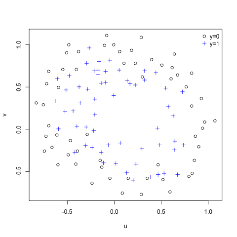
The idea of “fitting” is to create a mathematical model, that will separate the circles from the crosses in the plot above by learning from the existing data. That will then allow to make predictions for a new u and v value, the probability of being a cross.

Theory

Hypothesis is:

\h_\theta(x) = g(\theta^T x) = \frac{1}{ 1 + e ^{- \theta^T x} }

Regularization is all about loosen up the tight fit, avoiding over-fitting and thus obtain a more generalized fit, that more likely will work better on new data(for doing predictions).

For that we define the cost function, with an added generalization parameter that blunts the fit, like so:

J(\theta) = \frac{1}{m} \sum_{i=1}^m [(-y)log(h_\theta(x)) - (1 - y) log(1- h_\theta(x))] + \frac{\lambda}{2m} \sum_{i=1}^n \theta^2

lambda is called the regularization parameter.

The iterative theta updates using Newton’s method is defined as:

\theta^{(t+1)} = \theta^{(t)} - H^{-1} \nabla_{\theta}J

And the gradient and Hessian are defined like so(in vectorized versions):

\nabla_{\theta}J = \frac{1}{m} \sum_{i=1}^m (h_\theta(x) - y) x + \frac{\lambda}{m} \theta

H = \frac{1}{m} \sum_{i=1}^m [h_\theta(x) (1 - h_\theta(x)) x^T x] + \frac{\lambda}{m} \begin{bmatrix} 0 & & & \ & 1 & & \ & & … & \ & & & 1 \end{bmatrix}

Implementation

Lets first define the functions above, with the added generalization parameter:

# sigmoid function
g = function (z) {
  return (1 / (1 + exp(-z)))
} # plot(g(c(1,2,3,4,5,6)), type="l")

# build hight order feature vector
# for 2 features, for a given degree
hi.features = function (f1,f2,deg) {
  n = ncol(f1)
  ma = matrix(rep(1,length(f1)))
  for (i in 1:deg) {
    for (j in 0:i)    
      ma = cbind(ma, f1^(i-j) * f2^j)
  }
  return(ma)
} # hi.features(c(1,2), c(3,4),2)
# creates: 1 u v u^2 uv v^2 ...

# hypothesis
h = function (x,th) {
  return(g(x %*% th))
} # h(x,th)

# derivative of J 
grad = function (x,y,th,m,la) {
  G = (la/m * th)
  G[1,] = 0
  return((1/m * t(x) %*% (h(x,th) - y)) +  G)
} # grad(x,y,th,m,la)

# hessian
H = function (x,y,th,m,la) {
  n = length(th)
  L = la/m * diag(n)
  L[1,] = 0
  return((1/m * t(x) %*% x * diag(h(x,th)) * diag(1 - h(x,th))) + L)
} # H(x,y,th,m,la)

# cost function
J = function (x,y,th,m,la) {
  pt = th
  pt[1] = 0
  A = (la/(2*m))* t(pt) %*% pt
  return((1/m * sum(-y * log(h(x,th)) - (1 - y) * log(1 - h(x,th)))) + A)
} # J(x,y,th,m,la)

Now we can make it iterate until convergence, first for lambda=1

# setup variables
m = length(mydata$u) # samples
x = hi.features(mydata$u, mydata$v,6)
n = ncol(x) # features
y = matrix(mydata$y, ncol=1)

# lambda = 1
# use the cost function to check is works
th1 = matrix(0,n)
la = 1
jiter = array(0,c(15,1))
for (i in 1:15) {
  jiter[i] = J(x,y,th1,m,la)
  th1 = th1 - solve(H(x,y,th1,m,la)) %*% grad(x,y,th1,m,la) 
}

Validate that is converging properly, by plotting the Cost(J) function against the number of iterations.

# check that is converging correctly
plot(jiter, xlab="iterations", ylab="cost J")

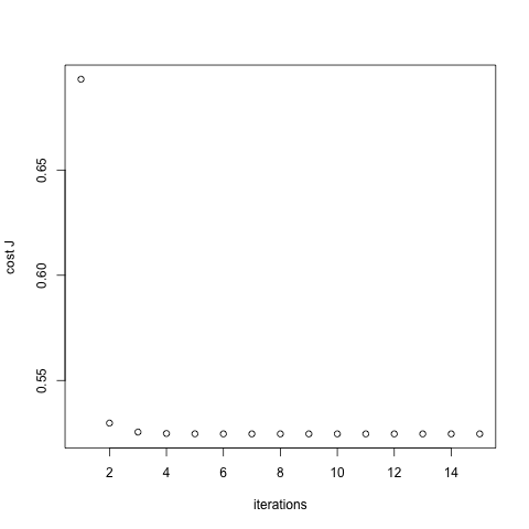
Converging well and fast, as is typical from Newton’s method.

And now we make it iterate for lambda=0 and lambda=10 for comparing fits later:

# lambda = 0
th0 = matrix(0,n)
la = 0
for (i in 1:15) {
  th0 = th0 - solve(H(x,y,th0,m,la)) %*% grad(x,y,th0,m,la) 
}

# lambda = 10
th10 = matrix(0,n)
la = 10
for (i in 1:15) {
  th10 = th10 - solve(H(x,y,th10,m,la)) %*% grad(x,y,th10,m,la) 
}

Finally calculate the decision boundary line and visualize it:

# calculate the decision boundary line
# by creating many points
u = seq(-1, 1.2, len=200);
v = seq(-1, 1.2, len=200);
z0 = matrix(0, length(u), length(v))
z1 = matrix(0, length(u), length(v))
z10 = matrix(0, length(u), length(v))
for (i in 1:length(u)) {
  for (j in 1:length(v)) {
    z0[j,i] =  hi.features(u[i],v[j],6) %*% th0
    z1[j,i] =  hi.features(u[i],v[j],6) %*% th1
    z10[j,i] =  hi.features(u[i],v[j],6) %*% th10
  }
}

# plots
contour(u,v,z0,nlev = 0, xlab="u", ylab="v", nlevels=0, col="black",lty=2)
contour(u,v,z1,nlev = 0, xlab="u", ylab="v", nlevels=0, col="red",lty=2, add=TRUE)
contour(u,v,z10,nlev = 0, xlab="u", ylab="v", nlevels=0, col="green3",lty=2, add=TRUE)
points(mydata$u[mydata$y == 0], mydata$v[mydata$y == 0])
points(mydata$u[mydata$y == 1], mydata$v[mydata$y == 1], col="blue", pch=3)
legend("topright",  c(expression(lambda==0), expression(lambda==1),expression(lambda==10)), lty=1, col=c("black", "red","green3"),bty="n" )

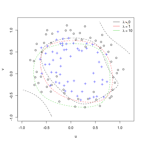
See that the black line (lambda=0) is the more tightly fit to the crosses, and as we increase the lambda values it becomes more loose(and more generalized) and consequently a better predictor for new unseen data.

References

• Thanks to Andrew Ng and OpenClassRoom for the great lessons.