Machine Learning Ex5.1 - Regularized Linear Regression

Exercise 5.1 Improves the Linear Regression implementation done in Exercise 3 by adding a regularization parameter that reduces the problem of over-fitting.

Over-fitting occurs especially when fitting a high-order polynomial, that we will try to do here.

With implementation in R.

Data

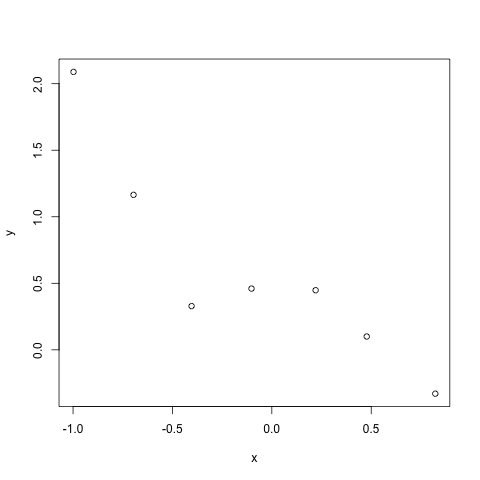
Here’s the points we will make a model from:

google.spreadsheet <- function (key) {
  library(RCurl)
  # ssl validation off
  ssl.verifypeer <- FALSE

  tt <- getForm("https://spreadsheets.google.com/spreadsheet/pub", 
                hl ="en_GB",
                key = key, 
                single = "true", gid ="0", 
                output = "csv", 
                .opts = list(followlocation = TRUE, verbose = TRUE)) 

  read.csv(textConnection(tt), header = TRUE)
}

# load the data
mydata = google.spreadsheet("0AnypY27pPCJydGhtbUlZekVUQTc0dm5QaXp1YWpSY3c")

# view data
plot(mydata)

Theory

We will fit a 5th order polynomial, so the hypothesis is:

h_\theta(x) = \theta_0 x_0 + \theta_1 x_1 + \theta_2 x_2^2 + \theta_3 x_3^3 + \theta_4 x_4^4 + \theta_5 x_5^5

With x_0 = 1

The idea of the regularization is to blunt the fit a bit, i.e. loosen up the tight fit.

For that we define the cost function like so:

J(\theta) = \frac{1}{2m} [\sum_{i=1}^m ((h_\theta(x^{(i)}) - y^{(i)})^2) + \lambda \sum_{i=1}^n \theta^2]

The Lambda is called the regularization parameter.

The regularization parameter added at the end will influence the exact cost values on all parameters. This will reflect in the search for the (\theta) parameters and consequently loosen up the tight fit.

After some math that is not shown here, the normal equations with the regularization parameter added, become:

\theta = (X^T X + \lambda \begin{bmatrix} 0 & & & \ & 1 & & \ & & … & \ & & & 1 \end{bmatrix} )^{-1} (X^T y)

Implementation

We will try 3 different lambda values to see how it influences the fit. Starting with lambda=0 where we can see the fit without the regularization parameter.

# setup variables
m = length(mydata$x) # samples
x = matrix(c(rep(1,m), mydata$x, mydata$x^2, mydata$x^3, mydata$x^4, mydata$x^5), ncol=6)
n = ncol(x) # features
y = matrix(mydata$y, ncol=1)
lambda = c(0,1,10)
d = diag(1,n,n)
d[1,1] = 0
th = array(0,c(n,length(lambda)))

# apply normal equations for each of the lambda's
for (i in 1:length(lambda)) {
  th[,i] = solve(t(x) %*% x + (lambda[i] * d)) %*% (t(x) %*% y)
}

# plot
plot(mydata)

# lets create many points
nwx = seq(-1, 1, len=50);
x = matrix(c(rep(1,length(nwx)), nwx, nwx^2, nwx^3, nwx^4, nwx^5), ncol=6)
lines(nwx, x %*% th[,1], col="blue", lty=2)
lines(nwx, x %*% th[,2], col="red", lty=2)
lines(nwx, x %*% th[,3], col="green3", lty=2)
legend("topright", c(expression(lambda==0), expression(lambda==1),expression(lambda==10)), lty=2,col=c("blue", "red", "green3"), bty="n")

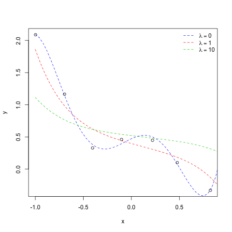
With the lambda=0 the fit is very tight to the original points (the blue line) but as we increase lambda, the model gets less tight(more generalized) and thus avoiding over-fitting.

References:

• Exercise 3, original Linear Regression implementation

• Thanks to Andrew Ng and OpenClassRoom for the great lessons.